A Sparse Coarse Space for VBD from Element Eigenmodes

VBD’s per-vertex 3×3 solve already gives the locally optimal descent direction — there is no leverage left inside a single block. So why does it still slow down on problems with high stiffness contrast? The answer turns out to be a story about what basis you descend in, and once that picture is in place the fix — a sparse coarse correction built from per-element eigenmodes — almost suggests itself.

Conditioning, geometrically

For a symmetric positive definite matrix in the 2-norm,

The quadratic energy $E(\mathbf{x}) = \tfrac{1}{2}\mathbf{x}^T A \mathbf{x}$ has level sets that are ellipsoids whose principal axes are the eigenvectors of $A$ and whose squared semi-axis lengths are $1/\lambda_i$. So $\kappa$ is literally the squared aspect ratio of the level-set ellipse. Big $\kappa$ means very elongated; $\kappa = 1$ means a sphere.

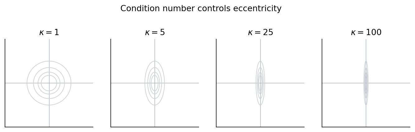
That ratio is exactly what governs CG’s convergence:

For a FEM stiffness matrix, $\kappa$ is at least as bad as the stiffness ratio between the stiffest and softest elements. A contrast of $10^6$ pushes the CG factor to $\approx 0.999$ — thousands of iterations to make a dent. Stiffness contrast is the standard way to wreck a global iterative solve.

But CG is not what VBD does. VBD is block coordinate descent, and for BCD, $\kappa$ is not the governing quantity.

Diagonal dominance is a different geometry

Partition $A$ into block-diagonal $D$ and off-diagonal $L + L^T$. Block Gauss-Seidel iterates with matrix $M = -(D+L)^{-1}L^T$, and its convergence rate is $\rho(M)$, controlled by block diagonal dominance — the size of each diagonal block $D_i$ relative to its incident off-diagonal entries.

This is a distinct quantity from $\kappa$. Geometrically:

• $\kappa$ controls the eccentricity of the energy ellipse — how elongated the level sets are.
• Diagonal dominance controls the alignment — how rotated those level sets are relative to your coordinate axes.

You can have a well-conditioned, nearly circular system whose principal axes are tilted 45° from the coordinate basis: BCD still zig-zags because each coordinate step cuts diagonally across the level sets. And you can have a horribly elongated system whose long axis is aligned with a coordinate axis: BCD walks straight down it in a sweep.

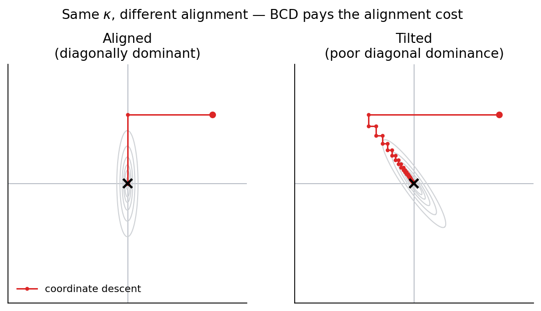
Same $\kappa = 25$ in both panels, completely different BCD experience. That distinction is why VBD does fine on uniformly stiff materials but stalls at interfaces: a soft vertex coupled to a stiff neighbor has small $D_i$ but a large off-diagonal entry on the stiff side. Local diagonal dominance breaks at the interface, regardless of the global condition number.

Every iterative method is a choice of descent basis

Once the picture is “an energy ellipse and a sequence of line searches,” every iterative method just becomes a strategy for picking the directions to search along. Three are well-established, plus a fourth that this post is building toward:

Eigenbasis. Diagonalize $A = Q \Lambda Q^T$ and change variables $\mathbf{z} = Q^T\mathbf{x}$. In the new coordinates, the energy decouples into independent parabolas $\sum_i \tfrac{1}{2}\lambda_i z_i^2 - \tilde b_i z_i$, and each one is solved in a single division. One sweep, done. The catch is finding $Q$ in the first place: an eigendecomposition costs $O(n^3)$, which is more expensive than the direct solve you were trying to avoid.

CG. CG does not try to find the eigenbasis directly. It builds its own basis adaptively, one vector per iteration, by taking matrix-vector products from the current residual:

Each new direction is $A$-conjugate to the previous ones, so progress in one direction is never undone in the next. In 2D, two iterations span the whole space and CG is exact. The directions are globally optimal given what CG has seen, but each is dense — forming the next Krylov vector takes a full matvec, and computing $\alpha_k$ takes a global inner product. That is the parallel bottleneck.

VBD (colored Gauss-Seidel). VBD picks the coordinate axes, in disjoint groups. Within a color, every vertex’s 3 coordinate axes are independent and can be solved in parallel via direct 3×3 inverses. The directions are sparse by construction (one vertex’s 3 axes touch only that vertex and its incident elements) so the local solves are embarrassingly parallel and there is no global reduction — but the basis is fixed in the coordinate system, regardless of where the actual eigenvectors of $A$ are pointing. When the principal axes are tilted, every coordinate step is partly orthogonal to the direction it should be going, and the iteration zig-zags.

Sparse local-eigen basis. What I am after: directions that are sparse like VBD’s (so the local solve and parallelism survive) but spectrally informed like CG’s (so each direction actually points along a principal axis of $A$). The element stiffness matrices give them to us for free, as we will see in a moment.

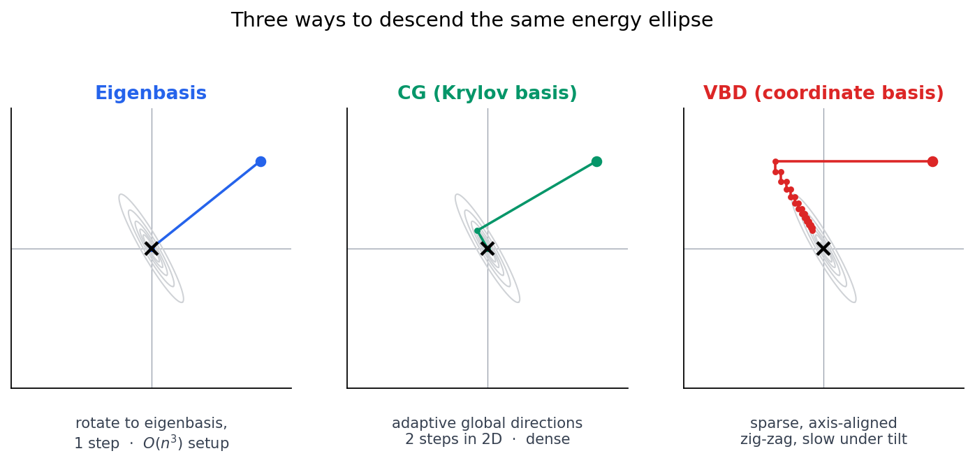
The three established strategies, stacked against the same tilted, ill-conditioned ellipse: eigenbasis walks straight in, CG takes two clean $A$-conjugate steps, VBD’s coordinate basis zig-zags down the long axis. The fourth strategy — sparse and spectrally informed — has no off-the-shelf solver to plot here yet; the rest of the post is what it would look like for VBD.

What an eigenbasis rebase buys

Zoom into the eigenbasis option for a moment. The reason it converges in one sweep is just that the change of variables $\mathbf{z} = Q^T \mathbf{x}$ rotates the ellipse so its principal axes line up with the new coordinate axes:

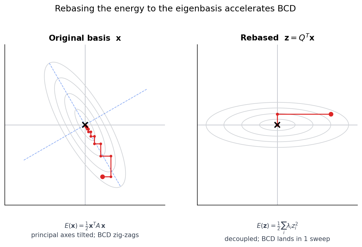
Same quadratic, same starting point, two coordinate systems. On the left the principal axes (dashed) sit at 30° from the coordinates and BCD ricochets between them. On the right, after applying $Q^T$ the contours line up with the new axes and one update of each coordinate lands at the minimum — the “sum of independent parabolas” decoupling $E(\mathbf{z}) = \frac{1}{2}\sum_i \lambda_i z_i^2$, each component solved by a single division $z_i^\star = \tilde b_i / \lambda_i$.

This is the upper bound on what any rebasing can buy. Every other strategy — CG’s adaptive Krylov directions, multigrid’s hierarchical bases, the usual preconditioners — is an approximation of the same trick at lower cost. For VBD we cannot afford the global $Q$, but the element stiffness matrices already hand us local $Q_e$’s for free; the rest of the post builds a cheap, sparse coarse correction on that observation.

VBD’s actual bottleneck

With graph coloring, every vertex of a given color is decoupled from every other vertex of that color. One color sweep is thousands of perfectly parallel 3×3 direct solves, each inverting its local Hessian exactly. There is no further leverage from rotating an individual block into its own eigenbasis — the direct $3\times 3$ inverse is already optimal in any basis.

So the bottleneck cannot be the local solve. It has to be inter-color communication. With $k$ colors and a mesh of diameter $d$, information needs $O(d/k)$ sweeps to cross the mesh: vertex $i$ updates in color 1, neighbor $j$ in color 2 sees the new residual the next sweep, vertex $l$ in color 1 sees $j$’s update the sweep after, and so on. The stiffer the inter-vertex coupling, the bigger the residual that bounces between colors — the BCD zig-zag, lifted from coordinate axes to entire colors.

That immediately tells me which modes I should care about: the ones that span colors and are stiff. Within-color modes are absorbed by the local solve; weak-coupling modes converge fine on their own.

Element eigenmodes as a free coarse basis

Every FEM element ships with its own stiffness matrix $K_e$ — $12\times 12$ for a linear tet, $9\times 9$ for a linear tri. Its eigendecomposition

is essentially free, and the columns of $Q_e$ are the element’s natural deformation modes (stretch along a fiber direction, shear, volumetric compression, etc.). Pick the stiffest few modes per element and stack them as columns of a tall, sparse matrix:

Each $\phi_j \in \mathbb{R}^{3N}$ is nonzero only on the vertices of its source element. Now solve a small reduced system at every outer iteration:

This is a deflation / coarse-space correction — it projects the residual into the span of the selected modes and solves optimally inside that span. Slotted into the VBD loop:

for each sweep:
    for each color:
        parallel_vertex_block_solves()   # standard VBD
    r = compute_residual()
    z = solve(P^T A P, P^T r)            # sparse coarse correction
    x += P @ z

The mental model: this is a physics-informed two-level method. The VBD color sweeps are the smoother — they handle high-frequency error perfectly. The coarse solve handles exactly the cross-color modes that the smoother is structurally incapable of resolving in a single sweep. Algebraic multigrid does the same trick, but pays a heavy setup phase to discover its coarse basis from algebraic heuristics. Here the basis is handed to us by the constitutive model.

Sparsity-wise: two columns of $P$ interact in $P^T A P$ only if their source elements share a vertex, so the coarse system is sparse along the element-adjacency graph. No global dense inner products like CG would need.

The cost of one direction

For a single sparse basis vector $\phi$, the optimal step along it is a 1D line search,

If $\phi$ has support on $k$ vertices, both products only touch a local neighborhood — $O(k\cdot\text{valence})$, not $O(n)$. For a nonlinear energy it is a couple of 1D Newton iterations on the same local support. Each individual direction is effectively free.

The cost lives in the count of columns of $P$, not in each column. Naïvely picking one mode per element gives $m \approx 5N$–$6N$ for a tet mesh, bigger than the original vertex system. That defeats the purpose.

What’s left to figure out

The construction is only useful if $P$ stays small. The pruning strategies that look most promising:

• Stiffness-contrast filter. Include modes only from elements whose stiffness deviates sharply from their neighbors — the interfaces where diagonal dominance actually breaks.
• Cross-color filter. Drop any mode whose support sits inside a single color. Those modes add no information the smoother is missing.
• Patch aggregation. Group neighboring elements and replace per-element top-modes with one patch-level mode — trade some spectral fidelity for far fewer columns.

I do not yet know which filter is sharpest in practice, or how few modes survive before the convergence gain disappears. But the structural picture is clean: the bottleneck is cross-color propagation, the analytical fix lives in element eigendecompositions we already have, and each individual sparse line search is nearly free. The whole game is picking the right small handful of directions.